7.5 Parametric Equations

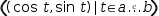
The coordinates of points that make up a curve can be defined by two expressions that depend on the same parameter. For example, the parametric equation of a circle is given by the equations x=cos t and y=sin t.

In Myron, a parametric sequence of points is defined by a tuple generator. The generator template consists of a point expression whose components capture the substance of parametric equations. The parameter is then bound to the generator's domain variable. If the generator domain is an interval expression whose limits are in turn bound to variable definitions, the adjusters associated with the variables can be used to control the values supplied to the parametric functions (see §7.5.2).

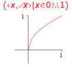
Exploratory plotting of parametric equations can be performed by situating a simple point expression whose components are single-valued functions as the template of a tuple generator whose domain variable is bound to the X-axis. Manipulating the extremities of the X-axis focuses the interval being plotted. These ideas are explored in §7.5.1

A simple point expression whose components are constant expressions is plotted as a position vector.

7.5.1 Simple Parametric Graph

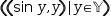
The simple function f(x)→√x is expressed parametrically by points (x, √x)ʋ. When the simple function is plotted, its x-range is determined by the limits of the x-axis. (See Figure 7.9.) However, when plotted as a parametric sequence, the x-range is determined by the generator domain, as in ((x, √x)ʋ|x∈0, 1, 0.1). If the generator domain is to be adjusted, its bounds and increment can be bound to adjusters. But note the extremes of the main axes are adjustable as well. This can be exploited to achieve the same simplicity as plotting a simple function by binding the generator domain to the X-axis using an axis domain: ((x, √x)ʋ|x∈𝕏).

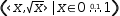
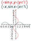
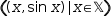
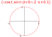
An axis domain only has a value in the context of the plotter. In the workspace, expressions with axis domains are not evaluable. Both axes are adjustable. To exploit this, an axis domain for the Y-axis is also available. For example, the parametric sequence ((x, sin x)|x∈𝕏) plots a sin wave from one end to the other of the x-axis. A related parametric sequence ((, sin y, y)|y∈𝕐) plots a rotated sin wave from one end of the y-axis to the other. Note the terms in the generator template have been reversed. A graph of these two parametric sequences is shown in Figure 7.9.

Figure 7.10 Generator domains bound to plotter axes

7.5.2 Parametric circle

The parametric graph of a circle is given by plotting ((, cos t, sin t)|t∈0, 2⋅ℼ+0.1, 0.1). The graph can be adjusted by plotting instead the four expressions a→0, c→0.1, b.→2⋅ℼ+c and ((, cos t, sin t)|t∈a, b, c). Figure 7.11 shows the graph of the equation. Note the definition of b must use an explicit real on the left to prevent parameter inference of c.